
Fake News Classification
In this tutorial I will be showing you guys how to develop and assess a fake news classifer using TensorFlow.
Initialization
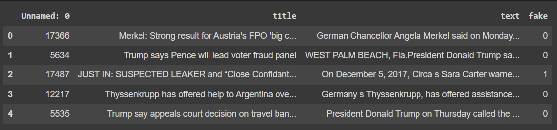
The data source we will be using comes from Kaggle. The following code will load in the neccessary packages along with our data. We can also explore our dataset a bit as well.
import tensorflow as tf
import numpy as np
import pandas as pd

train_url = "https://github.com/PhilChodrow/PIC16b/blob/master/datasets/fake_news_train.csv?raw=true"
train_df = pd.read_csv(train_url)

train_df.head()
Making our dataset
Now we’ll make a TensorFlow dataset to hold our data. The dataset will have two inputs, the article text and title, along with one output, whether its fake or not. First we’ll have to remove ‘stopwords’ in our data such as ‘the’ or ‘as’ which don’t really help us in our analysis. After we have constructed our dataset we’ll batch it in order to speed up training time.
import nltk
nltk.download('stopwords')

from nltk.corpus import stopwords

def make_dataset(df):
  #remove stopwords
  stop = stopwords.words('english')

  df['title'] = df['title'].str.lower()
  df['text'] = df['text'].str.lower()

  df['title'] = df['title'].apply(lambda x: ' '.join([word for word in x.split() if word not in (stop)]))
  df['text'] = df['text'].apply(lambda x: ' '.join([word for word in x.split() if word not in (stop)]))

  #make dataset
  data = tf.data.Dataset.from_tensor_slices(
    (
        {
            "title" : df[["title"]], #input
            "text" : df[["text"]]
        },
        {
            "fake" : df[["fake"]] #output
        }
    )
  )
  data = data.batch(100)
  return data
Great! We have just now constructed our TensorFlow dataset. Now lets take 20% of our data and use it as a validation set
data = make_dataset(train_df)
#shuffles the data
data = data.shuffle(buffer_size = len(data))

#20% of data being used for validation set
train_size = int(0.8*len(data))

train = data.take(train_size)
val = data.skip(train_size)

#checking number of entries
len(train), len(val)
(180, 45)
Now lets see the base rate of our model, which is the accuracy of a model that always makes the same guess.
train_df.shape[0], train_df['fake'].sum(), train_df['fake'].sum() / train_df.shape[0]
(22449, 11740, 0.522963160942581)
As we can see above the base rate accuracy of our model is about 52%.
Creating models
Now lets create some models using TensorFlow to answer the question: When detecting fake news, is it most effective to focus on only the title of the article, the full text of the article, or both?
Our first model will just focus on the title only.
from tensorflow.keras.layers.experimental.preprocessing import TextVectorization
import re
import string
from tensorflow import keras
from tensorflow.keras import layers
from tensorflow.keras import losses
Now we’ll need to vectorize, which is the process of turning text into numbers. Then it can be fed into our model.
#preparing a text vectorization layer for tf model
size_vocabulary = 2000

def standardization(input_data):
    lowercase = tf.strings.lower(input_data)
    no_punctuation = tf.strings.regex_replace(lowercase,
                                  '[%s]' % re.escape(string.punctuation),'')
    return no_punctuation

title_vectorize_layer = TextVectorization(
    standardize=standardization,
    max_tokens=size_vocabulary, # only consider this many words
    output_mode='int',
    output_sequence_length=500)

title_vectorize_layer.adapt(train.map(lambda x, y: x["title"]))
As you can see in the above code that we first turned all the words lower case and then removed punctuation.
Next we’ll construct the layers of our machine learning model. The embedding layer will take our vectorized title and put them in a vector space that can place similar words together or make paterns in the direction between words. The dropout layer will help prevent overfitting of our data. The pooling layer will give a wholistic view of the data instead of just patterns that are near each other. The dense layer will then gather our data together.
title_input = keras.Input( #input layer
    shape = (1,),
    name = 'title',
    dtype = 'string'
)

title_features = title_vectorize_layer(title_input)
title_features = layers.Embedding(size_vocabulary, 10, name = "title_embedding")(title_features) #10 dimension embedding layer
title_features = layers.Dropout(0.2)(title_features) #drop out 20% of data
title_features = layers.GlobalAveragePooling1D()(title_features)
title_features = layers.Dropout(0.2)(title_features)
title_features = layers.Dense(32, activation='relu')(title_features)

output = layers.Dense(2, name = 'fake')(title_features) #2 for fake or not fake

model1 = keras.Model(
    inputs = title_input,
    outputs = output
)

model1.summary()
Model: "model"
_________________________________________________________________
 Layer (type)                Output Shape              Param #
=================================================================
 title (InputLayer)          [(None, 1)]               0

 text_vectorization (TextVec  (None, 500)              0
 torization)

 title_embedding (Embedding)  (None, 500, 10)          20000

 dropout (Dropout)           (None, 500, 10)           0

 global_average_pooling1d (G  (None, 10)               0
 lobalAveragePooling1D)

 dropout_1 (Dropout)         (None, 10)                0

 dense (Dense)               (None, 32)                352

 fake (Dense)                (None, 2)                 66

=================================================================
Total params: 20,418
Trainable params: 20,418
Non-trainable params: 0
_________________________________________________________________
Now lets compile and train our model.
model1.compile(optimizer = "adam", #compile the model
              loss = losses.SparseCategoricalCrossentropy(from_logits=True),
              metrics=['accuracy']
)

history = model1.fit(train, #train the model
                    validation_data=val,
                    epochs = 10,
                    verbose = True)
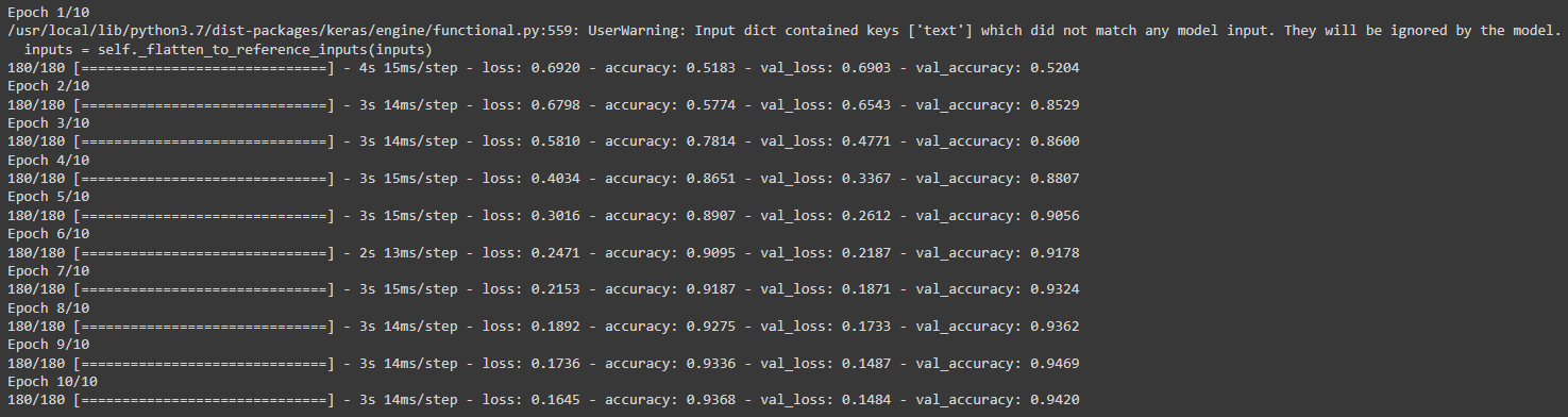
Our model1 has achieved a validation accuracy of 94% when just considering the title of the article.
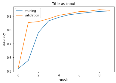
Plotting our model’s accuracies will also be very helpful.
from matplotlib import pyplot as plt

def plot_history(history, title = "type of input"):
  plt.plot(history.history["accuracy"], label = "training")
  plt.plot(history.history["val_accuracy"], label = "validation")
  plt.gca().set(xlabel = "epoch", ylabel = "accuracy")
  plt.title(f"{title} as input")
  plt.legend()

plot_history(history, title = "Title")
Onto our second model. This process will be similar to how we constructed our first model.
#same as our title model
vectorize_text = TextVectorization(
    standardize=standardization,
    max_tokens=size_vocabulary,
    output_mode='int',
    output_sequence_length=500)

vectorize_text.adapt(train.map(lambda x, y: x["text"]))

text_input = keras.Input(
    shape = (1,),
    name = 'text',
    dtype = 'string'
)

text_features = vectorize_text(text_input)
text_features = layers.Embedding(size_vocabulary, 10, name = "text_embedding")(text_features)
text_features = layers.Dropout(0.2)(text_features)
text_features = layers.GlobalAveragePooling1D()(text_features)
text_features = layers.Dropout(0.2)(text_features)
text_features = layers.Dense(32, activation='relu')(text_features)

output = layers.Dense(2, name = 'fake')(text_features)

model2 = keras.Model(
    inputs = text_input,
    outputs = output
)

model2.summary()
Model: "model_1"
_________________________________________________________________
 Layer (type)                Output Shape              Param #
=================================================================
 text (InputLayer)           [(None, 1)]               0

 text_vectorization_1 (TextV  (None, 500)              0
 ectorization)

 text_embedding (Embedding)  (None, 500, 10)           20000

 dropout_2 (Dropout)         (None, 500, 10)           0

 global_average_pooling1d_1   (None, 10)               0
 (GlobalAveragePooling1D)

 dropout_3 (Dropout)         (None, 10)                0

 dense_1 (Dense)             (None, 32)                352

 fake (Dense)                (None, 2)                 66

=================================================================
Total params: 20,418
Trainable params: 20,418
Non-trainable params: 0
_________________________________________________________________
model2.compile(optimizer = "adam", #compile the model
loss = losses.SparseCategoricalCrossentropy(from_logits=True),
metrics=['accuracy']
)
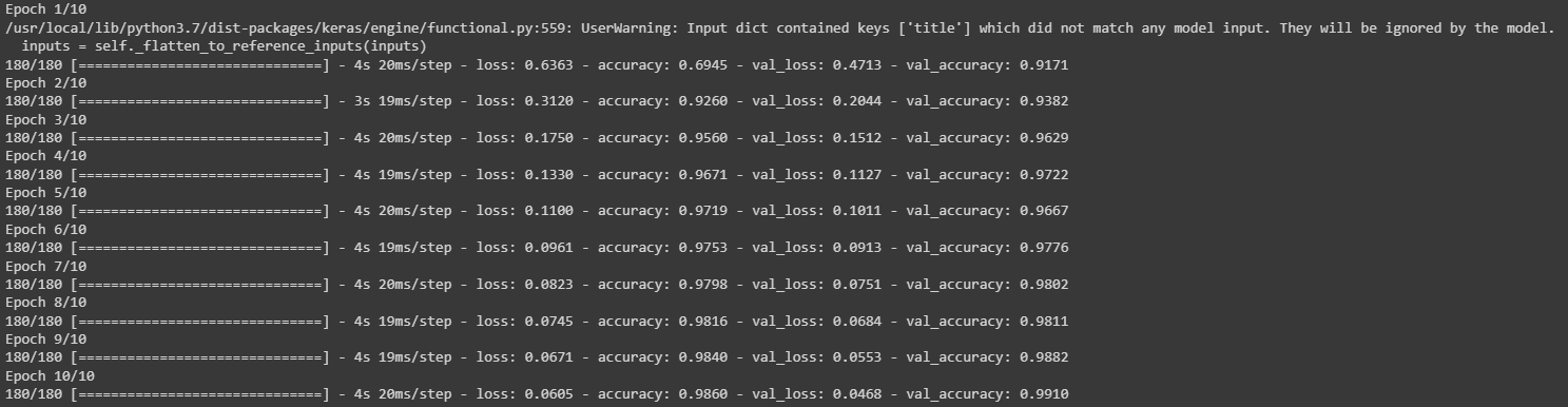
history = model2.fit(train, #train the model
validation_data=val,
epochs = 10,
verbose = True)
plot_history(history, title = 'Text')
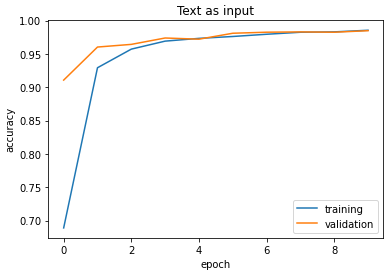
As we can see our model using only text had an accuracy of 98%. This is about 4% more than our first model. I hypothesize the reason why our accuracy is higher in this 2nd model is because of the amount of words used in an article’s body is much more than the amount of words used in the title.
Finally lets construct our 3rd model which will use both the title of an article and its text. To do this we can use the layers that we previously created for the other two models and concatenate them together.
#combined model
main = layers.concatenate([title_features, text_features], axis = 1)
#same as the previous models
main = layers.Dense(32, activation = 'relu')(main)
output = layers.Dense(2, name = 'fake')(main)
model3 = keras.Model(
    inputs = [title_input, text_input], #use both inputs
    outputs = output
)
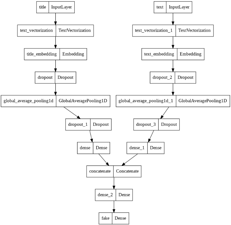
Instead of using model summary, lets instead use plot_model, which will give us a better look at the symmetry present.
keras.utils.plot_model(model3)
Next we’ll compile and train our model. This is similar to what we’ve done before with the other models.
model3.compile(optimizer = "adam", #compile the model
loss = losses.SparseCategoricalCrossentropy(from_logits=True),
metrics=['accuracy']
)
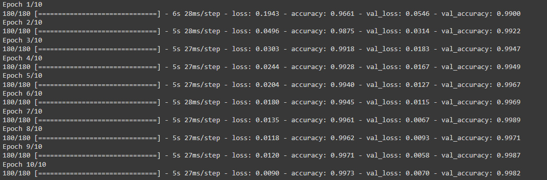
history = model3.fit(train, #train the model
validation_data=val,
epochs = 10,
verbose = True)
plot_history(history, title = 'Title and Text')
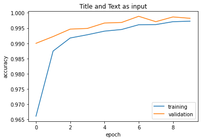
Our third model has garnered a 99% accuracy! From this we can conclude that the best way to classify fake news is to use both the article title and article text.
Model evaluation
Evaluating our best-performing model, model 3, against unseen data will be a good indicator to see how accurate it truly is.
test_url = "https://github.com/PhilChodrow/PIC16b/blob/master/datasets/fake_news_test.csv?raw=true"
test_df = pd.read_csv(train_url)

test = make_dataset(test_df)

model3.evaluate(test)
225/225 [==============================] - 3s 11ms/step - loss: 0.0087 - accuracy: 0.9976
[0.008745514787733555, 0.9975500106811523]
After testing our model against unseen data we have gotten a 99% accuracy which is the same as before.
Embedding visualization
Through the construction of our three models we used embedding layers. Now lets plot these embeddings and search for patterns.
weights = model3.get_layer('title_embedding').get_weights()[0]
vocab = title_vectorize_layer.get_vocabulary()

weights
array([[-0.00075599, -0.0049098 ,  0.00481388, ...,  0.00818873,
        -0.00486589,  0.00775187],
       [ 0.4359212 ,  0.37123716, -0.36165828, ..., -0.3338615 ,
         0.39441666, -0.3792474 ],
       [ 0.41503918,  0.33250818, -0.31997165, ..., -0.46919018,
         0.3793116 , -0.35538495],
       ...,
       [ 0.46491408,  0.44573432, -0.41716295, ..., -0.47136402,
         0.431214  , -0.5047367 ],
       [-0.28882578, -0.24557108,  0.32223096, ...,  0.2577063 ,
        -0.38530868,  0.33641776],
       [ 0.17766578,  0.24464168, -0.18960388, ..., -0.21405905,
         0.22452846, -0.30557597]], dtype=float32)
from sklearn.decomposition import PCA
#reducing dimensions so it can be plotted in 2d
pca = PCA(n_components = 2)
weights = pca.fit_transform(weights)
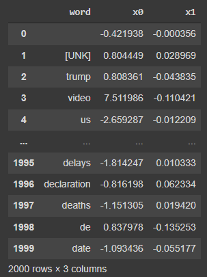
embedding_df = pd.DataFrame({
'word' : vocab,
'x0' : weights[:,0],
'x1' : weights[:,1]
})
embedding_df
import plotly.express as px
fig = px.scatter(embedding_df,
                 x = "x0",
                 y = "x1",
                 size_max = 2,
                 hover_name = "word",
                 title = "Word Embeddings in Article Titles")

fig.show()
By hovering on the right side of the middle of our plot we can see the words ‘dnc’ and ‘illegal’ together. This could mean that there are a lot of articles pointing to what the DNC does as illegal. On the very right hand we can see the words ‘gop’, ‘obama’s’, and ‘hillary’s’ together. This could mean that the GOP talks a lot about these Hillary and Obama, perhaps because they are both huge figures in the Democratic party.