
Exploring And Visualizing Climates Of Various Countries
In this Python tutorial we’ll use SQL to query a database we create along with making graphic visuals of the data using Plotly!
Creating our Database
Lets first make sure we have loaded in the necessary python packages for this.
#packages needed
import pandas as pd
from matplotlib import pyplot as plt
import numpy as np
import sqlite3
from plotly.io import write_html
Now lets create our database!
#creating the database
conn = sqlite3.connect
We have just created an empty database. In order for that database to actually be useful to us we need to load in the appropriate data.
#reading in the csv files
#reading in our temperature data in chunks
temps = pd.read_csv("temps_stacked.csv", chunksize = 100000)
#writing to the temperatures table in our database. first we will iterate through to create a FIPS code column which
#will help us later on when querying
for temp in temps:
temp["FIPS"] = temp["ID"].str[0:2]
temp.to_sql("temperatures", conn, if_exists = "append", index = False)
#reading in our stations data
stations_url = "https://raw.githubusercontent.com/PhilChodrow/PIC16B/master/datasets/noaa-ghcn/station-metadata.csv"
stations = pd.read_csv(stations_url)
stations.to_sql("stations", conn, if_exists = "replace", index = False)
#reading in our countries data and renaming some columns which will come in handy later
countries_url = "https://raw.githubusercontent.com/mysociety/gaze/master/data/fips-10-4-to-iso-country-codes.csv"
countries = pd.read_csv(countries_url)
countries = countries.rename(columns = {"FIPS 10-4" : "FIPS", "Name": "Country"})
countries.to_sql("countries", conn, if_exists = "replace", index = False)
Congrats! We have just created out database. Now lets check to see if we did it correctly.
#checking to see if the tables are correct
cursor = conn.cursor()
cursor.execute("SELECT name FROM sqlite_master WHERE type='table'")
print(cursor.fetchall())
#checking to see the columns of all our tables
cursor.execute("SELECT sql FROM sqlite_master WHERE type='table';")
for result in cursor.fetchall():
print(result[0])
conn.close()
Making a climate database querying function
Now that we have made our database how can we access certain data that we want? Well with this querying function we are able to do just that. We’ll be making a querying function that returns a panda dataframe telling us the temperature of the selected country and much more.
def query_climate_database(country, year_begin, year_end, month):
"""
This function takes in a country, a starting year, ending year, and month.
It then returns a pandas dataframe containg information such as station names and temperatures for the selected country.
"""
conn = sqlite3.connect("climate.db")
cmd = \
"""
SELECT S.name, S.latitude, S.longitude, C.country, T.id, T.month, T.year, T.temp
FROM temperatures T
LEFT JOIN stations S ON T.id = S.id
LEFT JOIN countries C ON T.fips = C.fips
WHERE C.country == '{0}' AND T.year >= {1} AND T.year <= {2} AND T.month == {3}
""".format(country, year_begin, year_end, month)
climate = pd.read_sql_query(cmd, conn)
climate.reset_index()
conn.close()
return climate
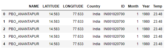
Lets see if we did this correctly with a test.
india = query_climate_database(country = "India",
year_begin = 1980,
year_end = 2020,
month = 1)
india.head()
Making a geographic scatter function
Now lets try making a geographic scatterplot function to better visualize our data on a map using plotly. For this we’ll need to import two more packages. Using the linear regression package from the sci-kit learn library we can also get the coefficients for the average change in temperature. Lets get started.
#the necessary modules
from sklearn.linear_model import LinearRegression
import plotly.express as px
import calendar
#our linear regression function
def coef(data_group):
#X is a df
x = data_group[["Year"]]
#y is a series
y = data_group["Temp"]
LR = LinearRegression()
LR.fit(x, y)
return LR.coef_[0]
def temperature_coefficient_plot(country, year_begin, year_end, month, min_obs, **kwargs):
"""
this function takes in a given country, starting year, ending year, month, minimum required years, and additional arguments for plot customization.
it returns an interactive plotly data visualization with labels, titles, and more interactive information.
"""
#get the specified dataframe
df = query_climate_database(country, year_begin, year_end, month)
#making sure stations that dont have the minimum amount of years aren't included
df['num_obs'] = df.groupby('NAME')['Year'].transform(len)
df = df[df['num_obs'] >= min_obs]
#creating our new yearly increase column in our df
coefs = df.groupby(["NAME", "Month","LATITUDE","LONGITUDE"]).apply(coef)
coefs = coefs.reset_index()
coefs.rename(columns={0: 'Estimated Yearly Increase'}, inplace = True)
coefs = coefs.round(4)
#making the figure
fig = px.scatter_mapbox(coefs,
lat = "LATITUDE",
lon = "LONGITUDE",
hover_name = "NAME",
color = "Estimated Yearly Increase",
color_continuous_midpoint = 0,
title = "Estimates of yearly temperature change in "+ calendar.month_name[month] \
+" for stations in "+ country +", years "+str(year_begin) + " - "+ str(year_end),
**kwargs)
return fig
Now that we’ve done that lets try it out by getting the yearly temperature changes in January from India between 1980 and 2020.
#choosing the colormap
color_map = px.colors.diverging.RdGy_r
fig = temperature_coefficient_plot("India", 1980, 2020, 1,
min_obs = 10,
zoom = 2,
mapbox_style="carto-positron",
color_continuous_scale=color_map)
fig.show()
write_html(fig, "india_plotly.html")
Since this is a function we created we can see this interactive geographic scatterplot with any country and time frame of our choosing.
Additional Visualizations
How does the average yearly temperature vary between two countries in a specific month?
def compare_two_countries(countries, year_begin, year_end, month, **kwargs):
"""
Given the desired countries (tuple or list of length 2), starting/ending year for the
data (int), a specific month (int), and additional keyword
arguments to be passed in to px.line(), we will return
a faceted line plot, divided by country, over time for the average
temperature in the specified month each year.
"""
#query two times, one for each country
df1 = query_climate_database(countries[0], year_begin, year_end, month)
df2 = query_climate_database(countries[1], year_begin, year_end, month)
#concatenate dataframes on top of each other
df = pd.concat([df1, df2], ignore_index = True)
#group by year and country and compute their average temperature
df = (df.groupby(["Year", "Country"])["Temp"].apply(np.mean)).reset_index()
#rename temp column
df = df.rename(columns = {"Temp" : "Temperature"})
#create adaptive title
title = f"{countries[0]} vs. {countries[1]} in
{calendar.month_name[month]}, Years {year_begin} - {year_end}
<br> <sup> Average Temperature in °C</sup>" #adds newline and subtitle
#lineplot
fig = px.line(df, x = "Year", y = "Temperature",
facet_col = "Country", #what to facet on
facet_col_spacing = .09, #increase horizontal spacing between facets
title = title,
**kwargs)
#change facet title to just be the country name
fig.for_each_annotation(lambda a:
a.update(text=a.text.replace("Country=","")))
fig.show()
Example of the Line Plot:
conn = sqlite3.connect("temps.db")
compare_two_countries(("United States", "Canada"), 1990, 2010, 2,
template = 'plotly_dark')
conn.close()
What is the distribution of temperatures like for a country over time in a specific month?
def boxplot_over_time(country, year_begin, year_end, month, **kwargs):
"""
Given the desired country (string), starting/ending year for the
data (int), a specific month (int), and additional keyword
arguments to be passed in to px.box(), we will return multiple box
plots of temperature for each year in the specified month, with added
hover data.
"""
#query the data base
df = query_climate_database(country, year_begin, year_end, month)
#rename the temp column
df = df.rename(columns = {"Temp" : "Temperature"})
#make adaptive title
title = f"Temperature Distribution in {country} in {calendar.month_name[month]}, Year {year_begin} - {year_end}"
#make the box plot
fig = px.box(df, x = "Year", y = "Temperature",
notched = True, #makes indents around the mean
title = title,
hover_data = ["Country", "Month"], #added hover data on the outliers
**kwargs)
fig.show()
Example of the Box Plot:
conn = sqlite3.connect("temps.db")
boxplot_over_time("Brazil", 2000, 2005, 3, template = 'plotly_dark')
conn.close()
Thank you for reading and following along!